What happens when the filter stops trusting the sensor

You built a Kalman filter for ICU biomarkers. You followed the textbook. State vector: position and velocity for each biomarker. Process model: constant velocity with noise. Measurement model: direct observation with Gaussian noise. You tuned the process noise Q and measurement noise R. You ran it on simulated data. It works beautifully, with smooth trajectories, accurate velocity estimates and clean separation of signal from noise.

Then you run it on real sensor data.

It works for the first 4 hours. Then the estimates start drifting. By hour 8, they are oscillating. By hour 12, they are useless. The filter is producing trajectories that bear no relationship to the patient's actual physiology. The velocity estimates are wild. The confidence intervals are narrow, because the filter thinks it is accurate, and the outputs are garbage.

What happened?

The sensor degraded. Electrochemical sensor membranes foul over time. Reference electrodes drift. Calibration accuracy decays between calibration cycles. A hemolyzed sample produced a potassium reading that was 1.2 mmol/L higher than reality. A lipemic specimen corrupted the bilirubin measurement. A drug interference made the creatinine assay report a value 30 percent above the true concentration.

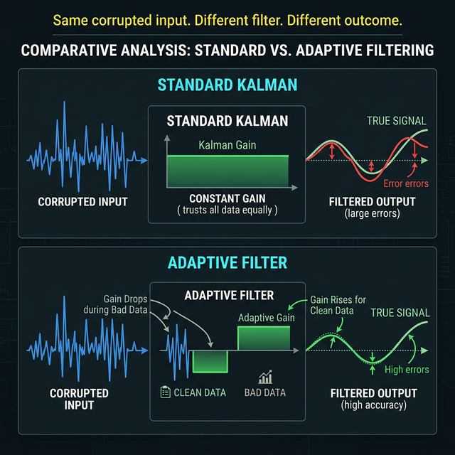
The filter did not know any of this. It kept trusting every measurement with the same confidence it gave to the first clean reading at hour zero. The measurement noise covariance R was a constant, a number you set during tuning and never changed. The Kalman gain stayed high. The filter pulled its state estimate toward every corrupted measurement. The estimates followed the noise into garbage.

This is the sensor reliability problem. And it is the reason that standard Kalman filtering has never been successfully deployed for continuous ICU biomarker trajectory estimation despite the mathematical framework being available since 1960.

1The reliability problem

Sensor degradation is predictable, not random.

Electrochemical sensors foul at known rates. The reaction surface accumulates proteins, fibrin, and cellular debris in a time-dependent process that follows well-characterized kinetics. If you know the sensor was last cleaned or replaced at time t₀, you can estimate the degradation at any subsequent time t with reasonable accuracy.

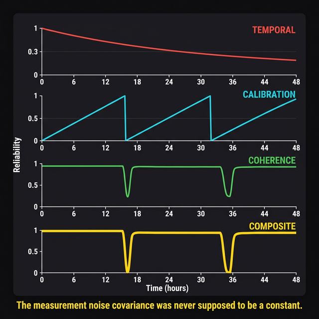
Calibration accuracy decays predictably between calibration cycles. A freshly calibrated analyzer has maximum accuracy. As time passes and environmental conditions drift, the accuracy degrades. The degradation profile is approximately linear for most clinical analyzers, with known slopes that depend on the analyte and the instrument type. Accuracy resets when the next calibration cycle occurs, creating a sawtooth pattern.

Physiological artifacts have signatures that can be detected. Hemolysis produces specific spectral changes that can be quantified by modern analyzers (hemolysis index). Lipemia similarly. Drug interferences are often predictable from the patient's medication list and the assay methodology. Cross-biomarker coherence (do the measurements make physiological sense together?) provides another layer of quality assessment.

Missing data is trivially detectable. The measurement either arrived or it did not.

All of this information is available. Standard Kalman filters have no mechanism to use it. The measurement noise covariance R is a constant, a fixed matrix. It does not change when the sensor degrades. It does not change when calibration drifts. It does not change when artifacts corrupt the measurement. It does not change when data goes missing. The filter is structurally incapable of modulating its trust in the data based on information it already has about the reliability of that data.

2The fix

The fix is one equation.

R(t) = R₀ / r(t)

R₀ is the baseline measurement noise covariance. The noise you would expect from a freshly calibrated, properly functioning sensor with a clean sample. This is the R you set during initial tuning. The textbook R.

r(t) is a scalar reliability function. It takes values from 0 to 1. When r(t) = 1, the sensor is perfectly reliable, and R(t) = R₀. Standard Kalman. When r(t) approaches 0, the sensor is unreliable, and R(t) grows toward infinity. The Kalman gain drops toward zero. The filter stops trusting the measurement and relies on its internal model to propagate the state estimate. When r(t) = 0 exactly (data missing), R(t) is infinite, the Kalman gain is exactly zero, the measurement is mathematically eliminated, and the filter runs in pure prediction mode.

One equation gives three limit behaviors, covering the entire degradation spectrum from perfect reliability to total sensor failure to missing data, handled by a single scalar function modulating a single parameter that the Kalman filter already has.

The elegance of this approach is that it requires no structural changes to the Kalman filter. The filter architecture stays exactly the same. The state transition model stays the same. The observation model stays the same. The prediction step stays the same. The only change is that R, instead of being a constant, becomes a function of time that reflects what you already know about the quality of the data arriving at the filter.

3Reliability decomposition

The reliability function r(t) decomposes into four factors:

r(t) = α_temporal × α_calibration × α_coherence × α_presence

α_temporal captures electrode degradation. Exponential decay from the last sensor replacement or cleaning. The decay constant is known for each sensor type and can be estimated from manufacturer specifications or empirical characterization.

α_calibration captures calibration proximity. Sawtooth function that equals 1 immediately after calibration and decays linearly until the next calibration cycle. Resets at each calibration event. The decay rate is known from analyzer specifications.

α_coherence captures physiological plausibility. If a potassium reading of 8.2 arrives while sodium is 140, chloride is 102, and the patient has no known reason for hyperkalemia, the reading may be an artifact (hemolyzed sample). Cross-biomarker coherence scoring detects these events by comparing the measurement against physiological expectations derived from the other biomarkers. Z-score based: how many standard deviations is this measurement from what the other biomarkers predict?

α_presence is a binary indicator. 1 if data arrived. 0 if data is missing. When α_presence = 0, r(t) = 0, R(t) = infinity, Kalman gain = 0, measurement eliminated. The filter continues in prediction mode until the next measurement arrives.

The composition is multiplicative. Any single factor reaching zero collapses total reliability to zero. A perfectly calibrated sensor (α_calibration = 1) that has been running for 72 hours without cleaning (α_temporal = 0.1) and just produced a measurement inconsistent with the other biomarkers (α_coherence = 0.2) has a composite reliability of 1 × 0.1 × 0.2 × 1 = 0.02. The filter treats this measurement as almost certainly unreliable and barely adjusts its state estimate. This is the correct behavior.

4Innovation-based process noise

There is a second equation that matters.

Q(t) = Q₀ × (1 + β × |innovation|)

The innovation is the difference between the predicted measurement and the actual measurement. In a well-tuned filter with a good model, the innovation should be small. When the innovation is large, one of two things happened: the measurement is bad, or the physiology changed.

The reliability function handles bad measurements. It reduces the influence of unreliable data. But what about the case where the measurement is reliable (α is high) and the innovation is still large? This means the patient's physiology changed in a way the process model did not predict. The filter's prediction was wrong because the physiology entered a new regime. Sepsis onset. Drug effect. Fluid bolus response. Something changed the dynamics.

When this happens, the filter needs to widen its process noise to track the new regime. Q(t) = Q₀ × (1 + β × |innovation|) does this automatically. Large reliable innovation widens the process uncertainty, which increases the Kalman gain on the next cycle, which makes the filter more responsive to subsequent measurements. The filter adapts to regime changes without external intervention.

Together, the two equations create a filter that does something no standard Kalman filter can do: it distinguishes between sensor failure and physiological change. When a large residual appears with low reliability, the filter suppresses the measurement (sensor failure). When a large residual appears with high reliability, the filter widens its process model and tracks the change (physiological regime shift). This distinction is critical in clinical monitoring where the consequences of confusing the two are catastrophic.

5What this looks like in practice

Imagine an ICU patient with a continuous lactate sensor (hypothetically, for now). Hour 0: sensor newly calibrated, all reliability factors near 1. The filter tracks lactate trajectory accurately, computing position and velocity in real time. The confidence interval is narrow.

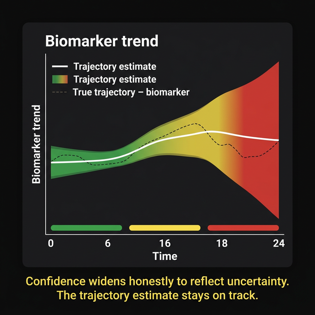
Hour 6: the sensor membrane has accumulated some fouling (α_temporal drops to 0.7). Calibration accuracy has decayed slightly (α_calibration drops to 0.85). R(t) increases. The Kalman gain decreases slightly. The filter relies a bit more on its model and a bit less on the raw measurement. The confidence interval widens slightly. The trajectory estimate remains accurate.

Hour 12: a blood sample shows hemolysis (α_coherence drops to 0.3). R(t) increases substantially. The Kalman gain drops. The filter essentially ignores this corrupted measurement and continues its trajectory estimate from the model prediction. The confidence interval widens further, honestly reflecting the uncertainty. But the trajectory does not jump to the corrupted value.

Hour 14: a fresh, clean measurement arrives. α_coherence returns to 1.0. R(t) decreases. The Kalman gain increases. The filter incorporates the new measurement, corrects any prediction drift, and the confidence interval narrows back toward operational accuracy.

Hour 18: the patient deteriorates rapidly (early sepsis). Lactate trajectory changes slope. The innovation spikes because the model predicted continuation of the previous trend. α_reliability is high (the sensor is working fine). Q(t) increases via the innovation-based term. The filter widens its process uncertainty, increases its tracking bandwidth, and follows the new trajectory.

No human intervention at any point. The filter computed everything automatically from information that was always available: sensor age, calibration timing, cross-biomarker coherence, and data presence. The mathematics did what a vigilant, computationally unlimited clinician would do: trust clean data, doubt corrupted data, and respond quickly when the patient changes.

6The one equation

R(t) = R₀ / r(t).

This is the core contribution of the Kunche Adaptive Estimator, published in preprint form (DOI: 10.22541/au.176313985.55971071/v1).

The measurement noise covariance was never supposed to be a constant. It was supposed to reflect everything you already know about whether you should trust the number arriving at the filter. The sensor age. The calibration status. The physiological plausibility. The simple fact of whether data arrived at all.

This information has always been available. In every clinical analyzer, every sensor system, every laboratory information system in every hospital in the world. The information was there. The filtering architecture just had no place to put it.

Now it does.

The measurement noise covariance R encodes trust. Making it a function of reliability is what the Kalman filter was always supposed to be, not an extension of it. Kalman gave us the architecture. The reliability function gives the architecture its senses.

The limit behaviors tell the complete story:

r = 1: Standard Kalman filtering. The sensor is reliable. Trust the data normally.

r approaching 0: Prediction mode. The sensor is degrading. Trust the model, doubt the measurement. Widen the confidence interval.

r = 0: Measurement eliminated. Data is missing. Ignore the measurement channel entirely. Propagate the prediction. Widen the uncertainty. Wait for the next measurement.

Three behaviors from one equation, with no switches, no if-then logic and no mode transitions. A continuous, differentiable function that handles the entire reliability spectrum through a single parameter that the Kalman filter was designed to accept.

The mathematics is published, the sensors exist, the hardware is trivial, and the patients are waiting. The information needed to compute reliability is already being recorded and discarded in every clinical laboratory in the world.

One equation, R(t) = R₀ / r(t), lets the filter decide how much to trust each sensor in real time. When the sensor degrades, the filter knows. When physiology changes, the filter adapts. No human tuning required.

The gap is neither mathematical nor technological; it is that nobody built the bridge between signal processing and clinical medicine, between what Kalman published in 1960 and what the ICU needs in 2026.

That bridge is one equation wide.